Excel Text Functions (II) - Extracting text strings using LEFT, RIGHT and MID

LEFT, RIGHT and MID are the three Excel Functions allow users to extract portions of strings from different positions.

(I) LEFT
LEFT returns a specified number of characters, starting from the left most character of the string:

In this example, we are using a sample text string "SYDNEYNSWAUSTRALIA" which is in cell A1.

First of all, we have to go to "Formulas" tab, select "Text" which activates a drop-down list, from which we highlight and select "LEFT".

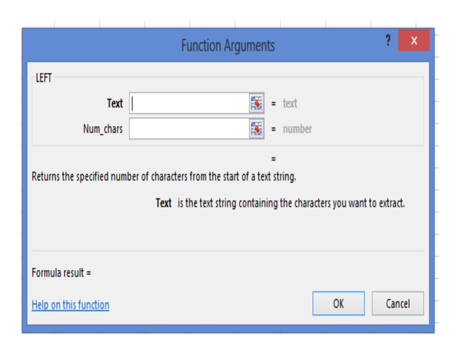
Once "LEFT" was selected, the "Function Arguments" dialog box will pop up:

User can either enter the text string directly into the "Text" box or clicking the small box at the right which will activate another dialog box as follows:

By clicking cell A1, Excel will put that cell reference into the "Text" box as shown below:

Next, user have to tell Excel how many characters from the left should be extracted, this is done by entering that number of characters into the "Num_chars" box. In our example, we enter 6 which means we will extract 6 characters from the left, following is the result:

(II) RIGHT

RIGHT returns a specified number of characters starting from the rightmost character of the string.

Similar to LEFT, user also access RIGHT by going to "Formulas" tab, select "Text" which activates the drop-down list, from which highlight and select "RIGHT", which will activate the "Function Arguments" dialog box as follows:

We are still using the text string in A1, the number of characters is 9, following is the result:

(III) MID

MID is the function that will return a specified number of characters starting from a specified position.

MID is also located under "Formulas" tab => "Text". From the drop-down list, we highlight and select "MID", which activates the Mid "Function Arguments" box:

We are still using the sample text in cell "A1" as our text string, the "Start_num" is 7, and the "Num_chars" is 3, following is the result:

Excel Text Functions (I) - Concatenating text strings

"CONCAT" (Excel 2016) or "CONCATENATE" (earlier versions) is the Excel function used to join two or more text strings into one.

The basic Syntax of CONCAT:

CONCAT (X1, X2, ...)

The arguments can be text strings or their respective cell references, and users can also add commas, hyphens, spaces, etc., to custom and format the resulting text. Following is an example:

Our arguments include 5 text strings located in cells A1 to A5, in between them we have added three spaces and one comma, following is the result:

The function can expand to concatenate data in cells of different columns:

By copying formula in E2, we can easily extend the concatenating actions towards other rows:

Pivot Table Basics - Calculated Fields

Users often need to perform data based calculations that are not in the original data set. This can be done in pivot table through the "Calculated Field". A calculated field is a virtual data field created by executing a calculation against existing fields in the pivot table, just like a new virtual column added to the data set.

Next, we will add a calculated field to the following pivot table:

Create a Calculated Field

Steps to create a calculated field:

(i) Select "Analyze" under the Pivot Table Tools
(ii) Select "Fields, Items & Sets"
(iii) From the drop-down menu select "Calculated Field".

(iv) The "Insert Calculated Field" dialog box will pop up

There are two input boxes inside the dialog screen. At the top is the "Name" field, which user can name the calculated field with a name of their choice, better appropriately to meet its function.

The one below is the "Formula" box, user can build their own formula by selecting the combination of data fields from the underneath "Fields" list box.

In this example, we create a calculated field to calculate the "Profit" for the property transactions:

We first select and double click the "Selling price" field, then enter the mathematical operator "- ", follow by "Purchase price"; then repeat the process again for each of the cost items to finalize the following formula into the formula box:

"Selling Price"-"Purchase Price"-"Stamp Duty"-"Conveyance"-"Improvement Cost"

Finally, click "O.K"

Then we can see the field under the name of "Sum of Profit" been added to Pivot Table:

Once the new calculated field was created, we can also find it in the "Fields" list box: